SCN Tutorial

Produced by Dianhui Wang & Matthew J. Felicetti

April 2022

1. Introduction

This tutorial will take you through the training and testing of Stochastic Configuration Networks (SCNs). SCNs are a novel randomized learner introduced by Dianhui Wang and Ming Li. SCN uses an incremental learning approach randomly assigning weights and bias for each idden layer of a neural network using a unique supervisory mechanism and adaptive scope setting. It is recommended that you have a read of the following paper before starting the tutorial:

D. Wang, M. Li, Stochastic configuration networks: Fundamentals and algorithms, IEEE Transactions on Cybernetics, 47(10)(2017) 3466-3479

The tutorial requires a computer with Matlab installed.

2. Basics

2.1 Neural Networks

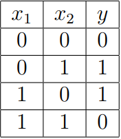
The XOR gate as shown in Figure 1 is a logic gate used in digital circuits. The XOR gate has the truth table as shown in Table 1 and as can be seen if both inputs (x₁ and x₂) are different a ’1’ is output ( y ), else if both inputs are the same a ’0’ is output. Whilst this concept may seem relatively simple, in terms of artificial intelligence this was a big problem for neural networks in the 1960s as the problem is not linearly separable. For us doing the tutorial, this is a good introduction problem as it is small and easy to follow.

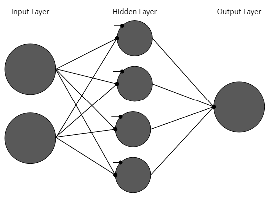
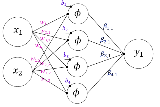
A feed-forward neural network is a network that moves in one direction, from input to output. After training an SCN model, the result will be a feed-forward model. A single hidden layer feed-forward model consists of three layers such that each layer feeds into the next via edges that have a weight between each node. The layers are the input, hidden and output. The input layer accepts the external data, whereas each node in the hidden layer applies a weighted sum of the input data using the hidden layers weights, and adds a bias term. This is then passed through an activation function to feed into the output layer. The output layer takes the weighted sum of the hidden layers outputs using the output weights, and then outputs the values that are used to accomplish some task. This is shown visually in Figure 2 .

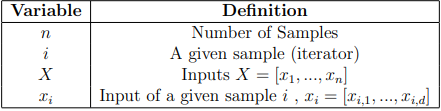
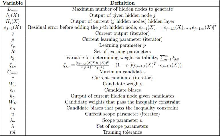
2.2 Notation

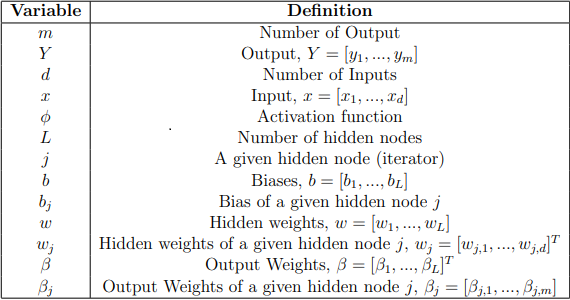
The notation for variables we will use in the model for this tutorial is given in Table 2 (variables are introduced as we go). With this, the SCN model can be given mathematically as follows:

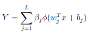
and can be added to our visual model in Figure 3.

2.3 Feed-forward Neural Networks

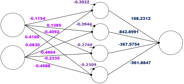
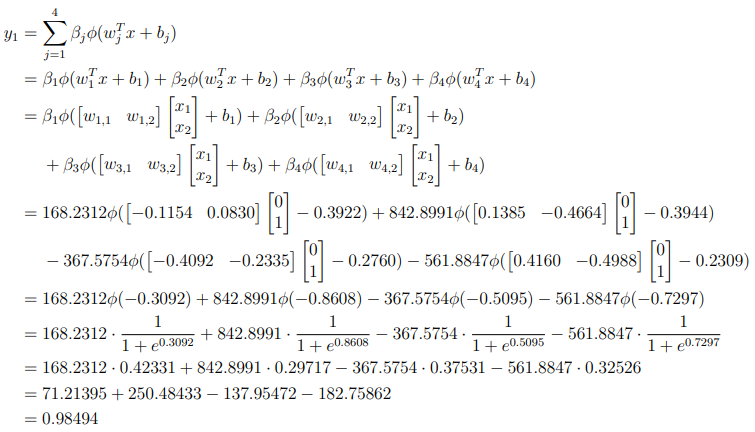
Our trained model then, has the values shown in Table 3 and we can then add these in our visual model in Figure 4.

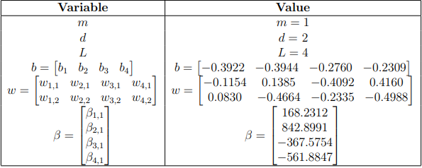
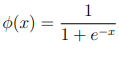
The activation function φ also needs to be established, for SCN any activation function can be used. In this example we will use the sigmoid activation function:

Let us now test this model by hand using the inputs x₁ = 0 and x₂ = 1:

From here we will test this using code. In matlab, set up a new script (Script 1) and introduce the variables:

		x = [0;1];
		w = [-0.1154 0.1385 -0.4092 0.4160 ; 0.0830 -0.4664 -0.2335 -0.4988];
		b = [-0.3922 -0.3944 -0.2760 -0.2309];
		beta = [168.2312; 842.8991; -367.5754; -561.8847];
		m = 1;
		y = 0;
                L = 4;

Then we can loop through each node, adding to our output each iteration and then displaying our output:

		...
		for j=1:L
		   y = y + 1/(1+exp(-(w(:,j).’*x+b(j))))*beta(j);
		end
		disp("y = " + y);

Running this, the output is given:

		y = 0.98623

We can see that this differs from our test by hand due to the accuracy of the computer being much greater due to us rounding.

From here it would be good to explore the other inputs, to do so we will modify the code such that all inputs can be evaluated at the same time. We also introduce and modify some variables as shown in Table 4.

Set up a new script (Script 2) and code as follows:

		X = [0 0 ;0 1; 1 0; 1 1];
		w = [-0.1154 0.1385 -0.4092 0.4160 ; 0.0830 -0.4664 -0.2335 -0.4988];
		b = [-0.3922 -0.3944 -0.2760 -0.2309];
		beta = [168.2312; 842.8991; -367.5754; -561.8847];
		m = 1;
		n = 4;
                L = 4;
		Y = logsig(bsxfun(@plus, X*w,b))*beta;
		for i=1:n
		   disp("y " + i + " = " + Y(i));
		end

Running, we get:

		y_1 = -0.0063887
		y_2 = 0.98623
		y_3 = 0.98665
		y_4 = -0.021382

2.4 Measuring Error

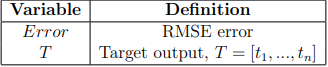
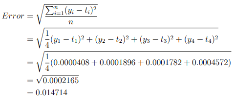
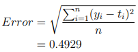
We have seen the output of the model, but we now need a way to determine the generalization cability of the model. To do this we require a measure of the error. We introduce some new notation given in Table 5 and the root mean square error formula:

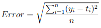
With this we have the target output T = 0, 1, 1, 0 and the output from our Matlab script Y = −0.0063887, 0.98623, 0.98665, −0.021382.

Hence to calculate:

Set up a new script (Script 3) and code as follows to calculate the error:

		X = [0 0 ;0 1; 1 0; 1 1];
		T = [0 ; 1 ; 1 ; 0];
		w = [-0.1154 0.1385 -0.4092 0.4160 ; 0.0830 -0.4664 -0.2335 -0.4988];
		b = [-0.3922 -0.3944 -0.2760 -0.2309];
		beta = [168.2312; 842.8991; -367.5754; -561.8847];
		m = 1;
		n = 4;
		Y = logsig(bsxfun(@plus, X*w,b))*beta;
		Error = sqrt(sum(sum( (Y-T).^2)/n));
		disp("Error = " + Error);

We should see the output:

		Error = 0.014714

which matches what we expect. With this we can now evaluate our SCN models we will be training in the next section.

3 Exercise 1

In this section we will train (and build) our SCN model using the XOR problem. Our training data will be the same as our testing data due to the size, but the following section will show a more appropriate approach to splitting the data. We will also introduce some more notation that we will use for the entire section in Table 6.

3.1 Constructive Network

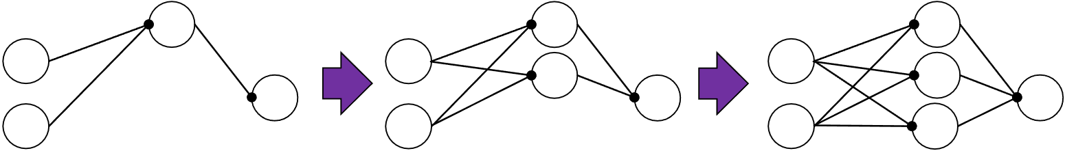
SCN training involves a constructive process, meaning that instead of the networks’ number of hidden nodes being fully defined at the start of training, the hidden nodes are iteratively added. This is shown in Figure 5. As can be seen in the figure, the number of weights, biases and output weights increase along side the hidden nodes every iteration. To start our network will not have any weights, biases or beta. Create a new Matlab script (Script 4) and add these variables:

		d = 2; m = 1; W = []; b = []; beta = [];

For our XOR problem we are going to set the maximum hidden nodes as L_max = 4 and we will use the variable j to track the number of nodes, which we will start this from 1:

		...
		j = 1; L_max = 4; 

To demonstrate the constructive approach, we will set all weights, biases and beta to 0. For the weights we will use an intermediate variables ( WC and bC ) to store them in , this will be important later:

		...
		while (j <= L_max)
		   WC = zeros(d,1);
		   bC = 0;
		   W = cat(2,W, WC);
		   b = cat(2,b, bC);
		   beta = zeros(j, 1);
		   disp("j = " + j);
		   disp("size(W) = " + mat2str(size(W)));
		   disp("size(b) = " + mat2str(size(b)));
		   disp("size(beta) = " + mat2str(size(beta)));
		   j = j + 1;
		end

Running this code we should get the output:

			j = 1
			size(W) = [2 1]
			size(b) = [1 1]
			size(beta) = [1 1]
			j = 2
			size(W) = [2 2]
			size(b) = [1 2]
			size(beta) = [2 1]
			j = 3
			size(W) = [2 3]
			size(b) = [1 3]
			size(beta) = [3 1]
			j = 4
			size(W) = [2 4]
			size(b) = [1 4]
			size(beta) = [4 1]

As can be seen the network can be constructed iteratively.

3.2 Generating Random Values

We have set up the constructive process, but now we must look at generating random values for the weights and biases. In SCN we use a uniform distribution to select from. To ensure that the values generated randomly match what is used in the tutorial, we will seed the values to a specific value, however in practice this is usually not desired. To seed add the following to Script 4 before the while loop:

		...
		rng(0);
		...

At this stage we will generate random values from −1 to 1, to do so we will use the rand function, however as it only generates values between 0 and 1 we will multiply by 2 and subtract 1. Modify the following variables in Script 4 to assign random values instead of zeros:

		...
		WC = 2*rand(d, 1)-1;
		bC = 2*rand(1, 1)-1;
		...

Note: This is how random values would be generated in random vector functional link (RVFL).

To test this we will change the disp s to as follows:

		...
		disp("j = " + j);
		disp("W = " + mat2str(W,5));
		disp("b = " + mat2str(b,5));
		...

Running this should display:

		j = 1
		W = [0.62945;0.81158]
		b = -0.74603
		j = 2
		W = [0.62945 0.82675;0.81158 0.26472]
		b = [-0.74603 -0.80492]
		j = 3
		W = [0.62945 0.82675 -0.443;0.81158 0.26472 0.093763]
		b = [-0.74603 -0.80492 0.91501]
		j = 4
		W = [0.62945 0.82675 -0.443 0.92978;0.81158 0.26472 0.093763 -0.68477]
		b = [-0.74603 -0.80492 0.91501 0.94119]

We are now able to generate random values.

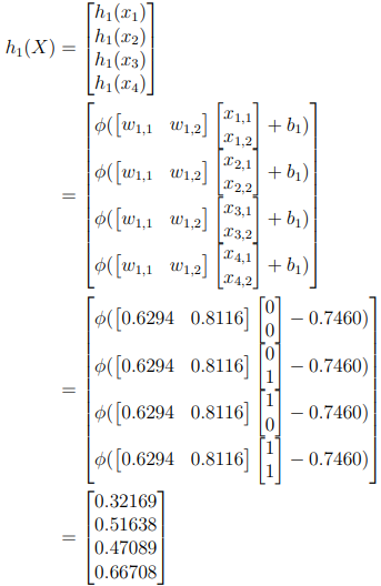
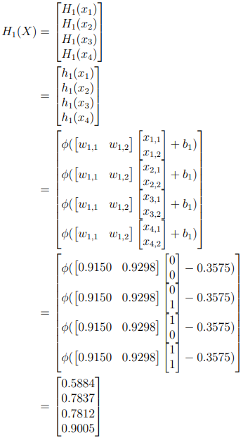
3.3 Inequality Constraint

Whilst we are able to generate random values for weights and biases, we also need a key feature of SCN, the inequality constraint. This is that the weights and bias generated do actually reduce the error. To determine this firstly we need to calculate the output of the hidden node given the hidden weights and biases. Given the very first iteration, we have w_1,1 = 0.6294, w_1,2 = 0.8116 and b₁ = −0.7460. With this we can calculate the output of the hidden node:

To perform this in our code, we need to add the inputs before the while loop:

		X = [0 0 ;0 1; 1 0; 1 1];
		...	

and then calculate the output of the hidden layer after generating the random values:

		...	
		hj = logsig(bsxfun(@plus, X*WC,bC));
		...	

From here we need to calculate ξ_j (ignoring candidates at the moment), to do so we need two more variables, learning parameter r_p and residual error e_j−1. For now we will fix p = 1, and r₁ = 0.9 (We will return to this later). The residual error at e₀ is T . With this we can calculate ξ_j :

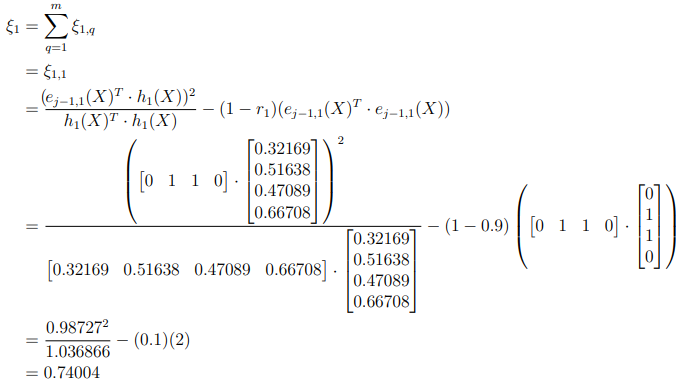
If all ξ_j,1, ..., ξ_j,m are greater than 0, then these weights and biases are suitable to use as they reduce the error. Now in this example we used r₁ = 0.9, but to create more opportunities for the values to be greater than 0, in SCN an iterative approach is taken, where the values of R used are R = [0.9, 0.99, 0.999, 0.9999, 0.99999, 0.999999]. We can now update (Script 4) to add the inequality constraint to our code for observation:

		d = 2; m = 1; W = []; b = []; beta = []; 
		j = 1; L_max = 4; n = 4; 
		X = [0 0; 0 1; 1 0; 1 1];
		T = [0; 1; 1; 0];
		rng(0);
		R = [ 0.9, 0.99, 0.999, 0.9999, 0.99999, 0.999999];
		ejminus1 = T;
		while(j <= L_max)
		   WB = []; bB = []; xiB = [];
		   WC = 2*rand(d, 1)-1;
		   bC = 2*rand(1, 1)-1;
		   hj = logsig(bsxfun(@plus, X*WC,bC));
		   for p = 1:length(R)
			  r_L = R(p);
			  xi = zeros(1, m);
			  for q = 1:m
				eq = ejminus1(:,q);
				xi(q) = ((eq’*hj)^2)/(hj’*hj) - (1 - r_L)*(eq’*eq);
			  end
			  xi_j = sum(xi);
			  disp("xi_j: " + xi_j)
			  if min(xi) > 0
				 disp("Passes")
				 W = cat(2,W, WC);
				 b = cat(2,b, bC);
			  else
				 disp("Fails")
			  end
		   end
		   beta = zeros(j, 1);
		   j = j + 1;
		end

This code demonstrates the inequality constraint, but we still need some more features before we can fully use it.

3.4 Multiple Candidates

So at this point we have the inequality constraint, but to take full advantage of this we need to generate more than one set of weights. In this step, we will generate a lot of different random weights and biases, called candidates (W_C and b_C). For this example we will use the number candidates C_max = 10. Add this before the while loop:

		C_max = 10; 
		...	

And then change the generation of weights as follows:

		...
		WC = 2*rand(d, C_max)-1;
		bC = 2*rand(1, C_max)-1;
		...

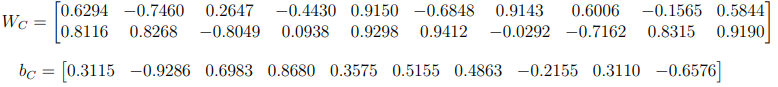
For the first iteration this will generate the random values shown below:

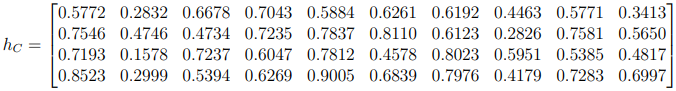
From here we will calculate the output of the hidden layer given the candidates, due to this we will change the notation from Hj to HC to indicate that we are using the candidates where each column is the output given a different set of candidates.

Replace and rename hj = logsig(bsxfun(@plus, X*WC, bC)); with hC = logsig(bsxfun(@plus, X*WC,bC)); , this should produce the following values for the first iteration:

We then need to check the inequality constraint for each candidate. If the candidate is suitable then we add it to a collection of weights and biases, W_B and b_B respectively. Further, we will store ξ_j in ξ_B if passing the inequality constraint.

• For candidate 1: ξ_j = 0.8121 > 0
• For candidate 2: ξ_j = 0.7516 > 0
• For candidate 3: ξ_j = 0.7651 > 0
• For candidate 4: ξ_j = 0.7921 > 0
• For candidate 5: ξ_j = 0.8283 > 0
• For candidate 6: ξ_j = 0.7321 > 0
• For candidate 7: ξ_j = 0.7818 > 0
• For candidate 8: ξ_j = 0.7535 > 0
• For candidate 9: ξ_j = 0.7729 > 0
• For candidate 10: ξ_j = 0.7467 > 0

As can be seen for this first hidden node, all pass the inequality constraint and so all the weights are added to W_B , the biases to b_B and ξ_j to ξ_B . But now we need to decide which one to use. To do this we sort the values of ξ_B and choose the highest value (i.e. reduces the error most), in this case this would be candidate 5, and so the weights 0.9150 and 0.9298, and bias 0.3575 would be chosen. The code (Script 4) can now be updated to include these changes:

		d = 2; m = 1; W = []; b = []; beta = []; 
		j = 1; L_max = 4; n = 4;
		X = [0 0; 0 1; 1 0; 1 1];
		T = [0; 1; 1; 0];
		rng(0);
		R = [ 0.9, 0.99, 0.999, 0.9999, 0.99999, 0.999999];
		ejminus1 = T;
		C_max = 10;
		while(j <= L_max)
		   WB = []; bB = []; xiB = [];
		   WC = 2*rand(d, C_max)-1;
		   bC = 2*rand(1, C_max)-1;
		   hC = logsig(bsxfun(@plus, X*WC,bC));
		   for p = 1:length(R)
			  r_L = R(p);
			  for c = 1 : C_max)
			      hc = hC(:,c);
			      xi = zeros(1, m);
			      for q = 1:m
			         eq = ejminus1(:,q);
			         xi(q) = ((eq’*hc)^2)/(hc’*hc) - (1 - r_L)*(eq’*eq);
			      end
			      xi_j = sum(xi);
			      if min(xi) > 0
			         xiB = cat(2,xiB, xi_j);
			         WB = cat(2,WB, WC(:,c));
			         bB = cat(2,bB, bC(:,c));
			      end 
			   end 
			   nC = length(xiB);
			   if  nC >= 1
				  break;
			   else
				  continue;			   
			   end
		   end
		   if  nC >= 1
			   [~, I] = sort(xiB, ’descend’);
			   W = cat(2,W, WB(:, I(1)));
			   b = cat(2,b, bB(:, I(1)));		   
		   else	   
			   disp("End Searching ...");
			   break			   
		   end		   
		   beta = zeros(j, 1);
		   j = j + 1;
		end

3.5 Output Weights

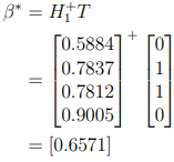
The output weights can be evaluated with every addition of hidden nodes by solving the least mean squares problem:

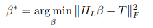
Where || ||_F represents the Frobenius norm. Practically, this can be achieved using the Moore- Penrose generalized inverse of H_L:

The Moore-Penrose generalized inverse can be implemented in Matlab using the pinv . So we now need to calculate the output of the hidden layer, for the first iteration we have:

From this we can calculate β:

Now that we have β, we can calculate the output

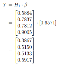
, the residual error

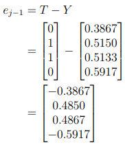
and the RMSE

We can now modify (Script 4) to include these changes:

		d = 2; m = 1; W = []; b = []; beta = []; 
		j = 1; L_max = 4; n = 4; 
		X = [0 0; 0 1; 1 0; 1 1];
		T = [0; 1; 1; 0];
		rng(0);
		R = [ 0.9, 0.99, 0.999, 0.9999, 0.99999, 0.999999];
		ejminus1 = T;
		C_max = 10;
		while(j <= L_max)
		   WB = []; bB = []; xiB = [];
		   WC = 2*rand(d, C max)-1;
		   bC = 2*rand(1, C max)-1 ;
		   hC = logsig(bsxfun(@plus, X*WC, bC));
		   for p = 1:length(R)
			  r_L = R(p);
			  for c = 1: C_max
			     hc = hC(:,c);
			     xi = zeros(1, m);
			     for q = 1:m
			        eq = ejminus1(:,q);
			        xi(q) = ((eq’*hc)^2)/(hc’*hc) - (1 - r_L)*(eq’*eq);
			     end
			     xi_j = sum(xi);
			     if min(xi) > 0
			        xiB = cat(2,xiB, xi_j);
			        WB = cat(2,WB, WC(:,c));
			        bB = cat(2,bB, bC(:,c));
			     end 
			   end 
			   nC = length(xiB);
			   if length(xiB) >= 1
				  break;
			   else
				  continue;			   
			   end
		   end
		   if nC >= 1
			   [~, I] = sort(xiB, ’descend’);
			   W = cat(2,W, WB(:, I(1)));
			   b = cat(2,b, bB(:, I(1)));
		   else	   
			   disp("End Searching ...");
			   break			   
		   end		   
		   Hj = logsig(bsxfun(@plus, X*[W],b));
		   beta = pinv(Hj)*T;
		   Y = Hj*beta;
		   ejminus1 = T - Y;
		   Error = sqrt(sum(sum( (Y-T).^2)/n));
		   disp("j=" + j + "RMSE=" + Error);
		   j = j + 1;
		end

3.6 Scope and Tolerance

Whilst we are able to now generate random weights and determine the output weights, we now need to consider that suitable weights may not be between -1 and 1. This is where the adaptive scope setting of SCN is applied. This feature is applied iteratively, such that if no suitable weights can be found, the scope is increased. The scope values used here are λ = [1, 5, 10, 30, 50, 100, 300, 500, 1000]. Another feature of SCN is the ability to stop training once a particular error is reached. This can also be added to our code, such that our main while loop will continue whilst the number of hidden nodes is less than or equal to the max or the tolerance is reached. In this we use a tolerance of tol = 0.00001.

This results in our final code (Script 4) for this problem:

		d = 2; m = 1; W = []; b = []; beta = []; 
		j = 1; L_max = 4; n = 4;
		X = [0 0; 0 1; 1 0; 1 1];
		T = [0; 1; 1; 0];
		rng(0);
		Lambdas = [1,5,10,30,50,100,300,500,1000];
		R = [ 0.9, 0.99, 0.999, 0.9999, 0.99999, 0.999999];
		ejminus1 = T;
		Error = sqrt(sum(sum( (ejminus1).^2)/n));
		tol = 0.00001;
		C_max = 10;
		while(j <= L_max) && (Error > tol) 
		   WB = []; bB = []; xiB = [];
		   for u = 1: length(Lambdas)
		      lambda_u = Lambdas(u);
		      WC = lambda_u*(2*rand(d, C_max)-1);
		      bC = lambda_u*(2*rand(1, C_max)-1);
		      hC = logsig(bsxfun(@plus, X*WC, bC));
		      for p = 1:length(R)
			  r_L = R(p);
			  for c = 1: C_max
			     hc = hC(:,c);
			     xi = zeros(1, m);
			     for q = 1:m
			        eq = ejminus1(:,q);
			        xi(q) = ((eq’*hc)^2)/(hc’*hc) - (1 - r_L)*(eq’*eq);
			     end
			     xi_j = sum(xi);
			     if min(xi) > 0
			        xiB = cat(2,xiB, xi_j);
			        WB = cat(2,WB, WC(:,c));
			        bB = cat(2,bB, bC(:,c));
			     end 
			   end 
			   nC = length(xiB);
			   if length(xiB) >= 1
		                  break;
			   else
		                  continue;			   
			   end
		       end
                       if length(xiB) >= 1
                              break;
                       else 
                              continue;
                       end
		   end
		   if nC >= 1
			   [~, I] = sort(xiB, ’descend’);
			   W = cat(2,W, WB(:, I(1)));
			   b = cat(2,b, bB(:, I(1)));
		   else	   
			   disp("End Searching ...");
			   break			   
		   end		   
		   Hj = logsig(bsxfun(@plus, X*[W],b));
		   beta = pinv(Hj)*T;
		   Y = Hj*beta;
		   ejminus1 = T - Y;
		   Error = sqrt(sum(sum( (Y-T).^2)/n));
		   j = j + 1;
		end
		disp("W=");
		disp(W);
		disp("b=");
		disp(b);
		disp("beta=");
		disp(beta);
		disp("RMSE=");
		disp(Error);

This code produces the randomly generated weights and biases, and the output weights using SCN. The output should be as shown:

		W=
		 0.9150 0.9004 0.8585 -0.9762
		 0.9298 -0.9311 -0.3000 -0.3258
		b=
		 0.3575 -0.7620 0.5075 -0.6952
		beta=
		 11.2564
		 14.5739
		 -20.4609
		 4.5386
		RMSE=
		 3.9752e-15

4 Exercise 2

4.1 Training and Testing Sets

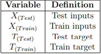
On the previous example, we only had four samples and hence used the same samples for training and testing. However, this is not ideal as we do not want the training to influence the testing. Hence we will introduce some new notation for the training and testing given in Table 7.

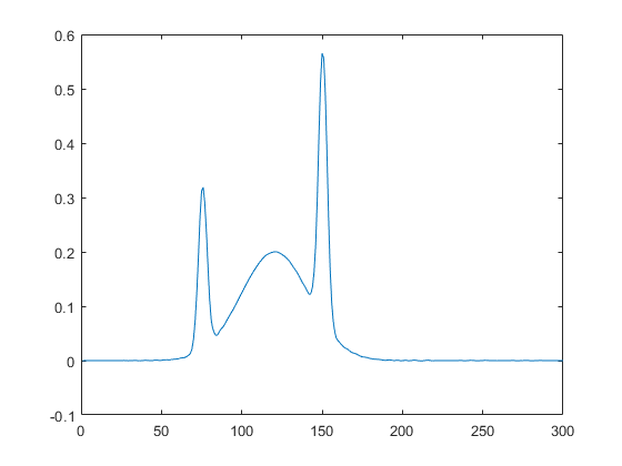
The dataset we will be using in this section is the real-valued function generated by:

We will generate 1000 samples from the uniform distribution from 0 to 1 for the training set. And we will generate 300 samples from a regularly spaced grid from 0 to 1 for the test set. Create a new script (Script 5) to generate the dataset, firstly clearing the workspace and setting the random number generator seed:

		clear;rng(0);

Then generate the training samples

		...
		Xtrain = rand(1, 1000)';
		Ttrain = 0.2*exp(-(10*Xtrain-4).^2) ...
		   +0.5*exp(-(80*Xtrain-40).^2)+0.3*exp(-(80*Xtrain-20).^2);

and then the testing samples

		...
		Xtest = linspace(0, 1, 300)';
		Ttest = 0.2*exp(-(10*Xtest-4).^2) ...
		   +0.5*exp(-(80*Xtest-40).^2)+0.3*exp(-(80*Xtest-20).^2);

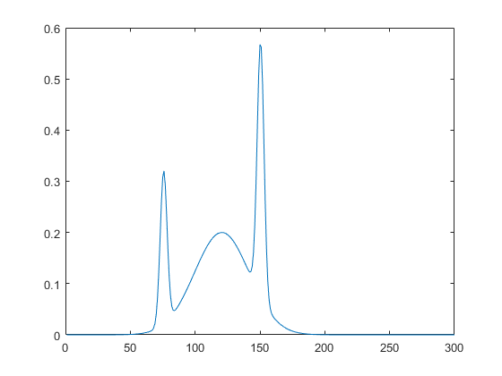
To confirm this works as expected plot Ttest

		...
		plot(Ttest);

and check that it matches what is shown in Figure 6.

We want to save this dataset now, so we do not need to create it every time:

		...
		save("tutorial_dataset");

Ensure you run this before continuing.

4.2 Training

We will be using the same code we used in the previous section, but with some changes, these changes include:

• Using our new dataset
• λ will now include 0.5
• Increasing the number of hidden nodes and candidates
• Storing the Error for each iteration
• Plotting the Error for each iteration
• Saving the model

Implement the code (Script 6) as shown to include these changes:

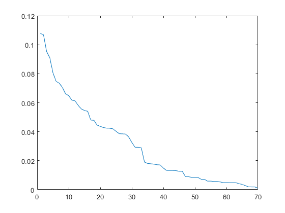
		clear;
		load("tutorial_dataset.mat");
		d = 1; m = 1; W = []; b = []; beta = []; j = 1;
		L_max = 100; n = 1000; C_max = 100;
		Lambdas = [0.5,1,5,10,30,50,100,300,500,1000];
		R = [ 0.9, 0.99, 0.999, 0.9999, 0.99999, 0.999999];
		ejminus1 = Ttrain;
		Error = sqrt(sum(sum( ejminus1.^2)/n));
		tol = 0.00001;
		rng(0);
		while (j <= L_max) && (Error > tol)
		   WB = []; bB = []; xiB = [];
		   for u = 1: length(Lambdas)
			  lambda_u = Lambdas(u);
			  WC = lambda_u*(2*rand(d, C max)-1);
			  bC = lambda_u*(2*rand(1, C max)-1) ;
			  hC = logsig(bsxfun(@plus, Xtrain*WC, bC));
			  for p = 1:length(R)
				 rp = R(p);
				 for c = 1: C_max ;
					hc = hC(:,c);
					xi = zeros(1, m);
					for q = 1:m
					   eq = ejminus1(:,q);
					   xi(q) = ((eq’*hc)^2)/(hc’*hc) - (1 - rp)*(eq’*eq);
					end
					xi_j = sum(xi);
					if min(xi) > 0
					   xiB = cat(2,xiB, xi_j);
					   WB = cat(2, W, WC(:,c));
					   bB = cat(2, b, bC(:,c));
					end
				 end
				 nC = length(xiB);
				 if nC >= 1
					break;
				 else
					continue;
				 end
			  end
			  if nC >= 1
				 break;
			  else
				 continue;
			  end
		   end
		   if nC>= 1
			  [~, I] = sort(xiB, ’descend’);
			  W = cat(2, W, WB(:, I(1)));
			  b = cat(2, b, bB(:, I(1)));
		   else
			  disp(’End Searching ...’);
			  break
		   end
		   Hj = logsig(bsxfun(@plus, Xtrain*[W],b));
		   beta = pinv(Hj)*Ttrain;
		   Y = Hj*beta;
		   ejminus1 = Ttrain - Y;
		   Error = sqrt(sum(sum( (Y-Ttrain).^2)/n));
		   ErrorTrain(j) = Error;
		   j = j + 1;
		end
		L = j - 1;
		plot(ErrorTrain);
		save("tutorial SCN model","W","b","beta","L");

Running this should produce the plot shown in Figure 7. This demonstrates that SCN is reducing the error every iteration.

4.3 Testing

To test the model we will create a new script, load the dataset and the model. Implement the code (Script 7) to test the model:

		clear
		load("tutorial_dataset.mat");
		load("tutorial_SCN_model.mat");
		n = 300;
		Y = logsig(bsxfun(@plus, Xtest*W,b))*beta;

Then we can display the error:

		...
		Error = sqrt(sum(sum( (Y-Ttest).^2)/n));
		disp("RMSE = " + Error);

This should produce:

		RMSE = 0.00028186

Demonstrating that the error is very small. Furthermore, we can plot the output:

		...
		plot(Y);

Doing so should produce the plot shown in Figure 8. We can see that this matches the target we saw earlier in Figure 6, demonstrating SCNs ability to solve this problem.

Concluding Notes

In this tutorial you have been able to train and test two different SCN models. Whilst this tutorial has tried to be as comprehensive as possible the following were not covered and hence you may want to try these yourself:

• Datasets with multiple outputs
• Classification problems

Further, some important remarks on extending and implementing yourself:

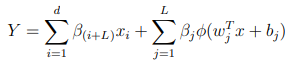
• Setting the hyperparameters (layers, tolerance, candidates, etc) can be difficult, and hence it is recommended that you apply a neural architecture search as outlined in:
  M. J. Felicetti, and D. Wang. "Deep stochastic configuration networks with optimised model and hyper-parameters." Information Sciences, 600 (2022) 431-441.
• In SCNs structure, we generally have a direct link between the input and the output layers, however for simplicity of implementation, this component is not included in this tutorial. Mathematically using the same notation as given in the tutorial this can be given as:
  
• In this implementation we used a uniform distribution is used to, however from recent works it is recommended that the normal distribution with an adaptive scale parameter is used as covered in:
  M. J. Felicetti, D. Wang, Deep Stochastic Configuration Networks with Different Random Sampling Strategies, Information Sciences, 607(2022) 819-830.


• Sample software with examples of using uniform, normal and logistic distributions can be found here:
  SCN Example - Distribution Examples

Furthermore, for the tutorial to ensure that the values produced were the same we seeded the random number generator. However to generate different random values every time you run the code you will need to remove rng(0);.